Fracture localization in Radiographs using machine learning.

Hypothesis

A convolutional neural network fine-tuned on labeled radiographs can localize fractures with useful precision, achieving IoU commonly above 0.5 on validation images, and improve further with data augmentation and careful fine-tuning.

Dataset

• Source: Labeled radiographs exported in YOLO format via Roboflow, organized into train, validation, and test splits. Each image has a paired .txt with class_id and normalized bbox (x_center, y_center, width, height). Post-cleanup removed MRI and mismatched labels to keep the distribution consistent with X-rays.
• Scale: Examples show 113 validation images analyzed in error analysis; overall training set larger. Labels describe a single “fracture” class.

What was done with the dataset

• Phase 1: Spot-checked labels by drawing YOLO boxes onto images to validate annotations.
• Phase 2: Built a tf.data pipeline to load, parse, resize, batch, shuffle, cache, and prefetch images and labels.
• Cleaning: Removed non-X-ray images and orphaned labels; scripted cleanup to maintain image–label parity.

Tools and methods

• Frameworks: TensorFlow and Keras for modeling and training. OpenCV and Matplotlib for visualization.
• Model: Transfer learning with MobileNetV2 as frozen backbone, custom regression head predicting bbox coordinates; later unfreezing for fine-tuning with low learning rate. Alternative architecture (ResNet50) considered for future work.
• Training regimen:
  • Stage 1 (feature extraction): ~15 epochs with backbone frozen.
  • Stage 2 (fine-tuning): +10 epochs with very low LR (e.g., 1e-6 to 5e-5) after unfreezing backbone.
• Augmentation: Random flips, rotations, zoom, brightness, and contrast to improve generalization and box precision.
• Experiment tracking: ClearML tasks used to name runs, log metrics, and store artifacts; best models retrieved from ClearML “Artifacts.”
• Evaluation: IoU between predicted and ground-truth boxes, qualitative overlays on test images, bulk error analysis producing per-image IoU and sorted outputs.
• Deployment demo: Local Streamlit app to interactively visualize predictions on uploaded images.

Experimental procedure (representative)

• Baseline model: 10 epochs, frozen backbone, saved as baseline; tracked in ClearML.
• Fine-tuned model: 15 epochs total plus fine-tuning stage with very low LR, saved and evaluated; multiple runs show expected stochastic variability in val_loss trajectory.
• Parameter tuning: Adjusted augmentation strength and fine-tuning LR; discussed batch size stability and optimizer choices (Adam vs. SGD, RMSprop).

Results

• Training/validation loss: Best val_loss typically in the mid–low 0.02x range; overfitting signals after peak epoch, motivating checkpointing at lowest val_loss rather than final epoch.

Baseline training

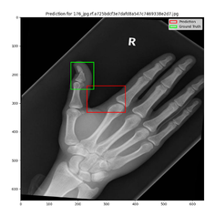
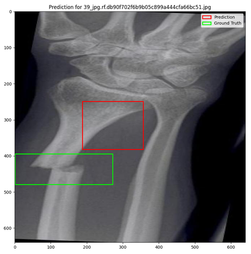
• IoU distribution: Validation-set IoU spanned 0.00 to ~0.53–0.67 across runs and subsets. Many cases exceeded 0.5 overlap, indicating correct localization; low-IoU cases revealed misses or poorly aligned boxes.
• Qualitative: ClearML sample grids and Phase 4/5 overlays show good localization on easier images and drift or misses on harder ones (blurry, small, atypical fractures).

Use of MobileNetV2

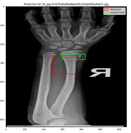
• Variability: Re-runs with identical settings produce small performance differences due to random initialization and shuffling; best-practice is to run several seeds and pick the best checkpoint.

Error analysis and insights

• High-IoU samples: Slight size or offset differences but strong localization.
• Medium-IoU samples: Consistent area but imprecise boundaries, suggesting benefit from augmentation and fine-tuning.
• Low-IoU samples: Missed or mislocalized boxes; prompts label audits and targeted data improvements.

Conclusion

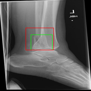
The transfer-learning approach successfully learned to localize fractures with meaningful precision on unseen images. Augmentation and careful fine-tuning improved robustness, while checkpointing at the lowest val_loss is key to capturing the true best model. The project demonstrates a complete ML lifecycle from data validation through training, analysis, and a minimal local deployment.

Final prediction

Recommended next steps

• Systematic checkpointing with ModelCheckpoint on val_loss minima.
• Additional data curation and label audits focused on low-IoU cases.
• Architecture exploration: ResNet50 or object-detection-specific heads.
• Extended augmentation and LR sweeps.
• Expand Streamlit UI for batch inference and side-by-side comparisons.

Source for dataset: Kaggle